Theory

 

1. Introduction

 

Numerical computer simulations of physical processes in acoustics allow for new results not available in the past due to complexity of simulations. 3D Acoustic Research has the goal to develop and implement complex mathematical numerical methods for loudspeaker analysis and design. We model the sound field produced by speaker in complex shape enclosure by 3D simulation. This allows for estimation of the speaker performance before its real construction.

 

Various mathematical speaker models exist which have zero problem dimension (i.e. sealed box or bass reflex calculators), or first order which take into account the variation of physical variables along one direction (i.e. 1D horn equation). However, a lot of acoustics enclosures such as horns, transmission lines, baffles etc have complex 3D shape, and thus simple models do not work well for them. For such systems only full 3D analysis is able to provide valuable result.

 

2. How that works

 

We use finite difference method for numerical modeling of sound field produced by the driver in the enclosure. The size of numerical grid element must be selected based on the complexity of the acoustic enclosure, the power of computational platform, the size of RAM and available time which restricts the simulation. In such type of mathematical problems one should take into account that reduction of grid size element drastically increases the full time of simulation. The last is proportionally to the number of 3D elements, and additionally increases due to the necessity of time step reduction which is related to the stability criteria of numerical method (Courant number).  These bring the method to the demand of memory, performance and the desire of highly parallel computational platform.

 

The calculation method we use is based on the solution of 3D wave equation for sound waves:

 

d^2(φ)/dt^2+ c^2* Δ (φ) =0

 

where φ is wave potential. This equation is rewritten in the form of finite differences to be solved on computer. This equation is solved in time and thus full information about sound field is obtained at arbitrary 3D point and arbitrary time. 

 

The driver enclosure is given as the set of rigid elements (walls) in the grid nodes reflecting the wave. The reflection condition is zero pressure gradient along the normal to the wall surface. Near the moving driver diffuser the boundary condition is given be the condition that velocity of particles in the wave is equal to the velocity of the diffuser. The motion of the diffuser is governed by Newton equation of motion under the presence of electromagnetic force, resilience of the surrounding, friction force, inertia, and the pressure force. The pressure around the driver can be non-uniform.

 

3. How that is visualized

 

3D Graphical  interface is developed for the representation of results after simulation is finished. In first release, almost arbitrary enclosure can be imported into 3D computational grid in the form of consequent 2D layers[1].  Driver parameters are set in conventional way via T/S parameters. The presentation of results is 3D. One can visualize the sound field, SPL, phase for given frequency at arbitrary point of computational domain.

 

Fig.1 shows complex acoustic enclosure known as back loaded horn which was imported into computational grid for simulation.

 

 

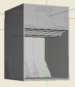
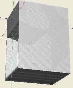
Fig 1.  Back loaded horn

 

After simulation is done for the given frequency range sound wave is shown (Fig.2), 3D distribution of RMS pressure level and phase (Fig.3).  For the enclosure in Fig.1 the simulation was carried out on numerical grid of the size 180 x 150 x 150 elements, each element having size 1 x 1 x 1  cm. 

 

Representation of parameters is shown along a given surface which is the cross section of the computational domain. The cross section is given as arbitrary and can be moved by mouse, which automatically changes the visualized parameters. 3D interface allows watching the image at different viewing angles and with variation of the scale.

 

Moving the virtual microphone to any desired position allows to plot SPL curve vs. frequency at that point.

500 Hz

200 Hz

 

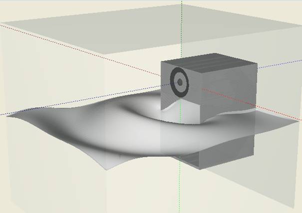
Fig.2. Sound wave field produced by horn

 

 

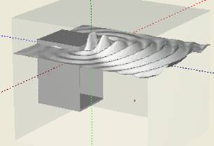
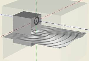
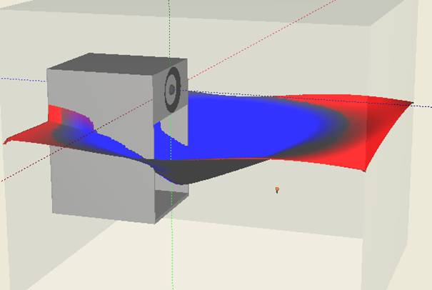
Fig. 3 .Sound field (2 kHz) at different cross-sections

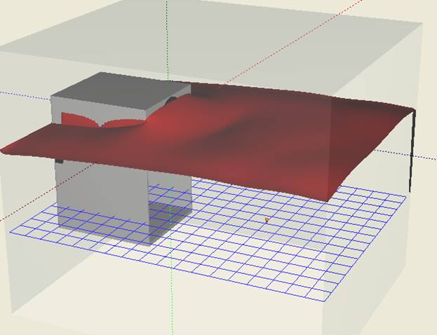
Fig. 4. SPL space distribution. Cross- section is shown by blue grid, and the surface level represents SPL.

 

 

 

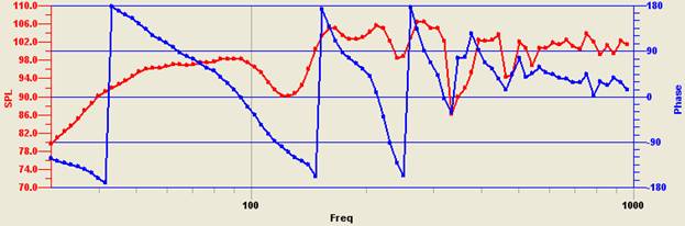
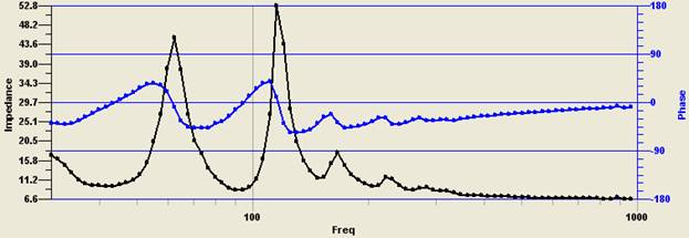
Fig. 5. SPL and given microphone position and impedance

 

4. Computations on CUDA

 

The development of CUDA parallel computational platform essentially expands the capabilities of numerical method for 3D modeling and design of acoustic systems.

 

Users buying the graphic card with CUDA support will receive the ability to accelerated the simulation in several dozen times (in first software release CUDA option is not included).

 

For graphic cards with CUDA support of middle cost (i.e. NVIDIA GTX 260) we were able to achieve the acceptable results with total computational time of around 30 min. The platform used will also allow in the future tocome across the results early considered as practically impossible (with further increase of grid and decrease of its element).

 

Based on our experiments the usage of CUDA platform at the given technology level allows to use the grid element size of the order of 1 cm. Such accuracy in many cases is enough for modeling of acoustic system in low and mid range frequency (up to 1 kHz), if the width of internal channels of the enclosure is bigger than 1 cm.

 

The examples in Figs.1-3 were calculated with CUDA on numerical grid 180 x 150 x 150 elements along 3 coordinates with the size of 1 cm. For NVIDIA GTX260 graphic card the simulation in the range of 20-1000 Hz with 1/6 octave step and integration time 60 mc for each frequency the simulation took 10 min 38 sec. We consider such result as good for practical usage if the instrument developed for design of acoustic systems.

 

We have developed two computational cores: one based on CUDA and another one without CUDA. The second core is written in C++ and compiled in Visual Studio 2008, runs on one processor core of personal computer without parallel threading. Also we do not used SSE optimization for the second core.

 

The comparison of two computational platforms (with CUDA and single CPU core) is shown in Table 1. It shows acceleration factor of about x27 for the given card.

 

Table.1 Acceleration factor, NVIDIA GTX260 with respect to Pentium 2.4 GHz  (single core)

 

Grid	64x64x64	128x128x128	256x256x256	512x400x400	512x400x400
Acceleration on CUDA	x2.1	x12	x25	X27	x28

 

 

5. Comparison with experiment

 

See our papers in News, where the modeling is compared with real measurements.